Gibbs Sampling

This example presents an illustration of the MLFM to learn the model

\[\dot{\mathbf{x}}(t)\]

We do the usual imports and generate some simulated data

import numpy as np
import matplotlib.pyplot as plt
from pydygp.probabilitydistributions import (Normal,
                                             GeneralisedInverseGaussian,
                                             ChiSquare,
                                             Gamma,
                                             InverseGamma)
from sklearn.gaussian_process.kernels import RBF
from pydygp.liealgebras import so
from pydygp.linlatentforcemodels import GibbsMLFMAdapGrad

np.random.seed(15)


gmlfm = GibbsMLFMAdapGrad(so(3), R=1, lf_kernels=(RBF(), ))

beta = np.row_stack(([0.]*3,
                     np.random.normal(size=3)))

x0 = np.eye(3)

# Time points to solve the model at
tt = np.linspace(0., 6., 9)

# Data and true forces
Data, lf = gmlfm.sim(x0, tt, beta=beta, size=3)

# vectorise and stack the data
Y = np.column_stack((y.T.ravel() for y in Data))

logpsi_prior = GeneralisedInverseGaussian(a=5, b=5, p=-1).logtransform()
loggamma_prior = Gamma(a=2.00, b=10.0).logtransform() * gmlfm.dim.K
beta_prior = Normal(scale=1.) * beta.size

fitopts = {'logpsi_is_fixed': True, 'logpsi_prior': logpsi_prior,
           'loggamma_is_fixed': False, 'loggamma_prior': loggamma_prior,
           'beta_is_fixed': False, 'beta_prior': beta_prior,
           'beta0': beta,
           }

nsample = 100
gibbsRV = gmlfm.gibbsfit(tt, Y,
                         sample=('g', 'beta', 'x'),
                         size=nsample,
                         **fitopts)

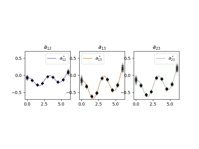
Learning the Coefficient Matrix

The goal in fitting models of dynamic systems is to learn the dynamics, and more subtly learn the dynamics of the model independent of the state variables.

aijRV = []
for g, b in zip(gibbsRV['g'], gibbsRV['beta']):
    _beta = b.reshape((2, 3))
    aijRV.append(gmlfm._component_functions(g, _beta))
aijRV = np.array(aijRV)

# True component functions
ttd = np.linspace(0., tt[-1], 100)
aaTrue = gmlfm._component_functions(lf[0](ttd), beta, N=ttd.size)

# Make some plots
inds = [(0, 1), (0, 2), (1, 2)]
symbs = ['+', '+', '+']
colors = ['slateblue', 'peru', 'darkseagreen']

fig = plt.figure()
for nt, (ind, symb) in enumerate(zip(inds, symbs)):

    i, j = ind

    ax = fig.add_subplot(1, 3, nt+1,
                         adjustable='box', aspect=5.)
    ax.plot(ttd, aaTrue[i, j, :], alpha=0.8,
            label=r"$a^*_{{ {}{} }}$".format(i+1, j+1),
            color=colors[nt])
    ax.plot(tt, aijRV[:, i, j, :].T, 'k' + symb, alpha=0.1)

    ax.set_title(r"$a_{{ {}{} }}$".format(i+1, j+1))
    ax.set_ylim((-.7, .7))
    ax.legend()

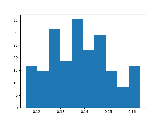
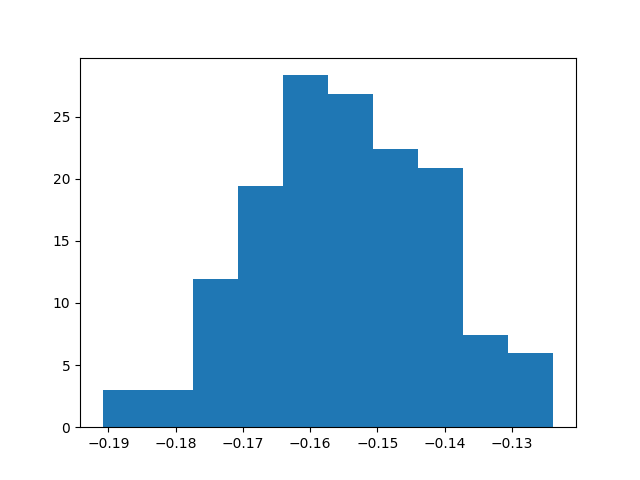
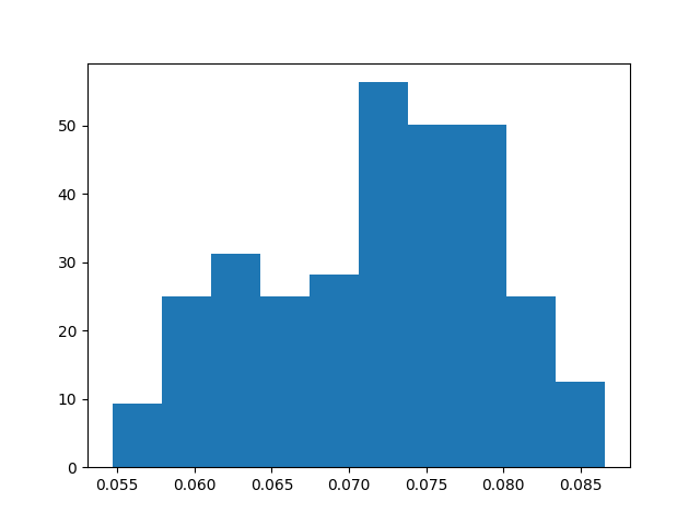
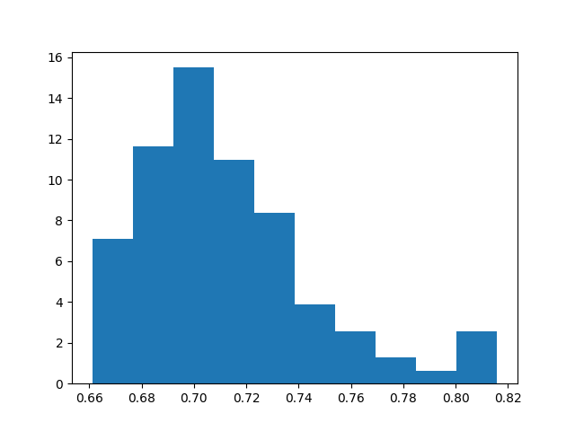
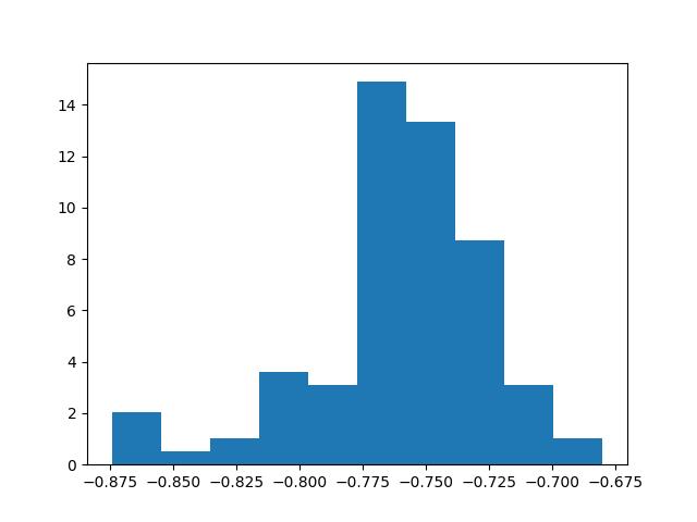
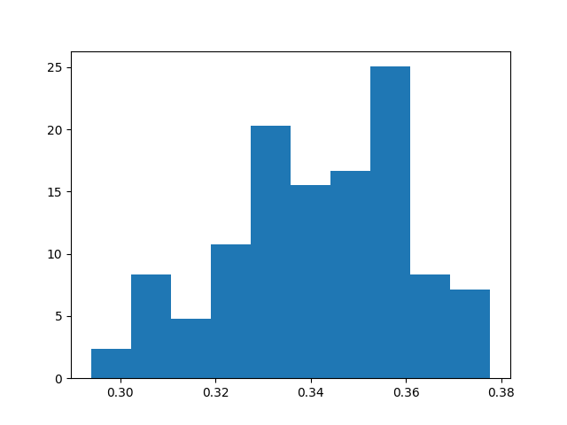
for i in range(gibbsRV['beta'].shape[-1]):
    fig, ax = plt.subplots()
    ax.hist(gibbsRV['beta'][:, i], density=True)

plt.show()

• 
• 
• 
• 
• 
• 
• 

Total running time of the script: ( 0 minutes 9.494 seconds)