Basic MAP Estimation

This note descibes how to carry out the process of carrying out MAP parameter estimation for the MLFM using the Adaptive Gradient matching approximation. This uses the MLFMAdapGrad object and so our first step is to import this object.

import numpy as np
import matplotlib.pyplot as plt
from scipy.integrate import odeint
from pydygp.linlatentforcemodels import MLFMAdapGrad
from sklearn.gaussian_process.kernels import RBF
np.random.seed(17)

Model Setup

To begin we are going to demonstate the model with an ODE on the unit sphere

\[S^{2} = \{ x \in \mathbb{R}^3 \; : \; \| x \| = 1 \},\]

which is given by the initial value problem

\[\dot{\mathbf{x}}(t) = \mathbf{A}(t) \mathbf{x}(t), \qquad \mathbf{x}_0 \in S^2,\]

where the coefficient matrix, \(\mathbf{A}(t)\), is supported on the Lie algebra \(\mathfrak{so}(3)\). We do this by representing the

\[\mathbf{A}(t) = \sum_{d=0}^3 \beta_{0d}\mathbf{L}_d + \sum_{r=1}^R g_r(t) \sum_{d=1}^3 \beta_{rd}\mathbf{L}_d,\]

where \(\{\mathbf{L}_d \}\) is a basis of the Lie algebra \(\mathfrak{so}(3)\). The so object returns a tuple of basis elements for the Lie algebra, so for our example we will be interested in so(3)

from pydygp.liealgebras import so
for d, item in enumerate(so(3)):
    print(''.join(('\n', 'L{}'.format(d+1))))
    print(item)

Out:

L1
[[ 0.  0.  0.]
 [ 0.  0. -1.]
 [ 0.  1.  0.]]

L2
[[ 0.  0.  1.]
 [ 0.  0.  0.]
 [-1.  0.  0.]]

L3
[[ 0. -1.  0.]
 [ 1.  0.  0.]
 [ 0.  0.  0.]]

Simulation

To simulate from the model we need to chose the set of coefficients \(\beta_{r, d}\). We will consider the model with a single latent forcing function, and randomly generate the variables \(beta\)

pydygp.linlatentforcemodels.MLFMAdapGrad.sim()

g = lambda t: np.exp(-(t-2)**2) * np.cos(t)  # single latent force
beta = np.random.randn(2, 3)

A = [sum(brd*Ld for brd, Ld in zip(br, so(3)))
     for br in beta]

ttd = np.linspace(0., 5., 100)
x0 = [1., 0., 0.]
sol = odeint(lambda x, t: (A[0] + g(t)*A[1]).dot(x),
             x0,
             ttd)

The MLFM Class

mlfm = MLFMAdapGrad(so(3), R=1, lf_kernels=(RBF(), ))

x0 = np.eye(3)

# downsample the dense time vector
tt = ttd[::10]
Data, _ = mlfm.sim(x0, tt, beta=beta, latent_forces=(g, ), size=3)

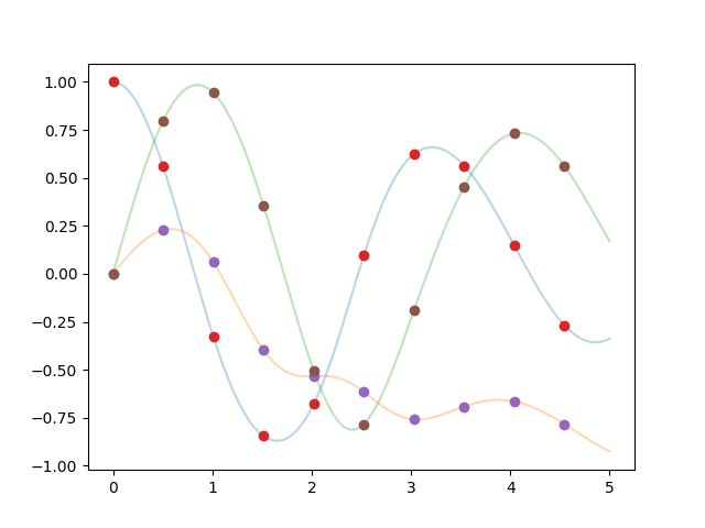
fig, ax = plt.subplots()
ax.plot(ttd, sol, '-', alpha=0.3)
ax.plot(tt, Data[0], 'o')

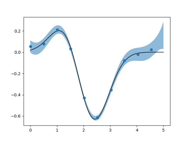
Latent Force Estimation

Y = np.column_stack(y.T.ravel() for y in Data)
res = mlfm.fit(tt, Y, beta0 = beta, beta_is_fixed=True)

# predict the lf using the Laplace approximation
Eg, SDg = mlfm.predict_lf(ttd, return_std=True)

# sphinx_gallery_thumbnail_number = 2
fig2, ax = plt.subplots()
ax.plot(ttd, g(ttd), 'k-', alpha=0.8)
ax.plot(tt, res.g.T, 'o')
for Egr, SDgr in zip(Eg, SDg):
    ax.fill_between(ttd,
                    Egr + 2*SDgr, Egr - 2*SDgr,
                    alpha=0.5)

plt.show()

Total running time of the script: ( 0 minutes 2.091 seconds)