Approximate Density

When using the method of successive approximation we construct a regression model

\[p(\mathbf{x} \mid \mathbf{g}, \boldsymbol{\beta}) = \mathcal{N}( \mathbf{x} \mid \mathbf{P}^{M} \boldsymbol{\mu}_0, \alpha \mathbf{I})\]

The idea is to construct an approximation to this density by introduction each of the successive approximations

\[\mathbf{z}_{i} = \mathbf{P}\mathbf{z}_{i-1},\]

the idea being that knowing the complete set of approximations \(\{ z_0,\ldots,z_M\}\) we can solve for the latent variables by rearranging the linear equations, instead of manipulating the polynomial mean function.

For this conversion to work we need to introduce a regularisation parameter \(\lambda > 0\) and then define \(\mathcal{N}( \mathbf{z}_{i} \mid \mathbf{P}\mathbf{z}_{i-1}, \lambda \mathbf{I})\), once we do this we can write log-likelihood of the state variables

\[\log = -\frac{\lambda}{2} \sum_{i=1}^{M} \left( \mathbf{z}_{i-1}^{\top}\mathbf{P}^{\top}\mathbf{P}\mathbf{z}_{i-1} - 2\mathbf{z}_{i}^{\top}\mathbf{P}\mathbf{z}_{i-1} \right)\]

Now the matrices \(\mathbf{P}\) are linear in the parameters which means that after vectorisation they can be represented as

\[\operatorname{vec}(\mathbf{P}) = \mathbf{V}\mathbf{g} + \mathbf{v}_0\]

Note

The matrices \(\mathbf{P}\) and their affine representations are most easily written compactly using kronecker products, unfortunately these are not necessarily the best computational representations and there is a lot here that needs refining.

Linear Gaussian Model

We take a break in the model to now discuss how to start putting some of the ideas discussed above into code. For the Kalman Filter we are going to use the code in the PyKalman package, but hacked a little bit to allow for filtering and smoothing of independent sequences with a common transition matrix.

import numpy as np
from pydygp.liealgebras import so
from sklearn.gaussian_process.kernels import RBF
from pydygp.linlatentforcemodels import MLFMSA
np.random.seed(123)
def _get_kf_statistics(X, kf):
    """ Gets
    """
    # the mean, cov and kalman gain matrix
    means, cov, kalman_gains = kf.smooth(X)
    # pairwise cov between Cov{ z[i], z[i-1]
    # note pairwise_covs[0] = 0  - it gets ignored
    pairwise_covs = kf._smooth_pair(covs, gains)

    S0 = 0.
    for m, c in zip(means[:-1], covs[:-1]):
        S0 += c + \
              (m[:, None, :] * m[None, ...]).transpose((2, 0, 1))
    S1 = 0.
    for i, pw in enumerate(pairwise_covs[1:]):
        S1 += pw + \
              (means[i+1][:, None, :] * \
               means[i][None, ...]).transpose((2, 0, 1))

    return S0.sum(0), S1.sum(0)


mlfm = MLFMSA(so(3), R=1, lf_kernels=[RBF(), ], order=5)
beta = np.array([[0.1, 0., 0.],
                 [-0.5, 0.31, 0.11]])
tt = np.linspace(0., 6., 15)
x0 = np.eye(3)
Data, g = mlfm.sim(x0, tt, beta=beta, size=3)

Expectation Maximisation

So we have introduced a large collection of unintersting latent variables, the set of successive approximations \(\{ z_0, \ldots, z_M \}\), and so we need to integrate them out. If we define the statistics

\[\boldsymbol{\Psi}_0 = \sum_{i=1}^{M} \langle \mathbf{z}_{i-1} \mathbf{z}_{i-1}^{\top} \rangle_{q(Z)}, \quad \boldsymbol{\Psi}_1 = \sum_{i=1}^{M} \langle \mathbf{z}_{i} \mathbf{z}_{i-1}^{\top} \rangle_{q(Z)}\]

Then the objective function of the M-step becomes

\[Q(\mathbf{g}, \mathbf{g}^{old}) = -\frac{1}{2} \mathbf{g}^{\top} \left( \mathbf{V}^{\top} (\boldsymbol{\Psi}_0 \otimes \mathbf{I}_{NK})\mathbf{V} + \lambda^{-1} \mathbf{C}^{-1} \right)\mathbf{g} - 2\]

More sensible place to start – the Kalman Filter performs the numerical integration

from pydygp.linlatentforcemodels import KalmanFilter

ifx = tt.size // 2  # index left fixed by the Picard iteration

mlfm._setup_times(tt, h=None)

A = mlfm._K(g[0](tt), beta, ifx)

init_conds = np.array([y[ifx, :] for y in Data])

# array [m0, m1, m2] with m0 = np.kron(Data[0][ifx, :], ones)
init_vals = np.kron(init_conds, np.ones(mlfm.dim.N)).T
final_vals = np.column_stack([y.T.ravel() for y in Data])

X = np.ma.zeros((mlfm.order, ) + init_vals.shape)  # data we are going to give to the KalmanFilter
X[0, ...] = init_vals
X[1, mlfm.order-1, ...] = np.ma.masked  # mask these values -- we have no data
X[mlfm.order-1, ...] = final_vals

NK = mlfm.dim.N*mlfm.dim.K
observation_matrices = np.array([np.eye(NK)]*3)

kf = KalmanFilter(initial_state_mean=init_vals,
                  initial_state_covariance=np.eye(NK)*1e-5,
                  observation_offsets=np.zeros((mlfm.order, NK, mlfm.dim.K)),
                  observation_matrices=observation_matrices,
                  transition_matrices=A,
                  transition_covariance=np.eye(NK)*1e-5,
                  transition_offsets=np.zeros(init_vals.shape),
                  n_dim_state=NK,
                  n_dim_obs=NK)

means, covs, k_gains = kf.smooth(X)

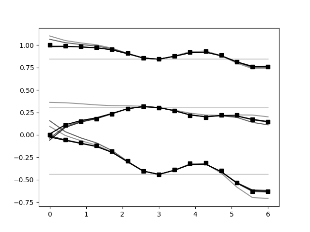
import matplotlib.pyplot as plt
fig, ax = plt.subplots()
for i, mean in enumerate(means):
    # unvectorise the column
    m = mean[:, 0].reshape((mlfm.dim.K, mlfm.dim.N)).T
    ax.plot(tt, m, 'k-', alpha=(i+1)/mlfm.order)
ax.plot(tt, Data[0], 'ks')
plt.show()

Total running time of the script: ( 0 minutes 0.092 seconds)